VIO-Metal
End-to-End VIO Pipeline on Apple Silicon with Metal GPU Acceleration

Visual-Inertial Odometry (VIO) is the problem of estimating a device’s position and orientation in 3D space by fusing camera images and inertial measurement unit (IMU) data. It underpins augmented reality, autonomous drones, and mobile robotics. State-of-the-art systems like VINS-Mono, OKVIS, and BASALT are typically built on CUDA or target embedded Linux platforms like NVIDIA Jetson. Almost none target Apple Silicon natively.
vio-metal is a from-scratch stereo VIO pipeline designed to exploit one of Apple Silicon’s most distinctive hardware features: the Unified Memory Architecture (UMA). On traditional discrete GPU systems, moving a 752×480 image from CPU RAM to GPU VRAM costs 2–5 ms per frame over PCIe. On Apple Silicon, CPU and GPU share the same physical DRAM. A MTLBuffer allocated with StorageModeShared is a single pointer — no copy, no staging buffer, no transfer latency. This changes the economics of GPU offloading: even sub-millisecond kernels are worth dispatching because the transfer overhead is effectively zero.
The project ships two parallel front-end pipelines: a CPU-only version using OpenCV for feature extraction, and a hybrid CPU+GPU version with five custom Metal compute shaders replacing the vision front-end. Both feed into a sliding-window nonlinear optimizer backed by Ceres Solver with Apple Accelerate providing the BLAS/LAPACK substrate.
This blog covers the full mathematical and engineering design: the Lie group foundations, the IMU preintegration theory, the factor graph formulation, and the GPU kernel implementations — including FAST corner detection, Harris response scoring, ORB descriptor extraction, stereo matching, and pyramidal KLT optical flow tracking on Metal.
1. The Mathematical Foundations: Rotations, Manifolds, and Lie Groups
Visual-inertial odometry lives on SE(3) — the special Euclidean group of rigid body transformations in 3D. Every component in the pipeline touches rotations: the IMU integrates angular velocity into incremental rotations, the optimizer differentiates cost functions with respect to orientation, and the reprojection factors rotate 3D landmarks into camera coordinates. Getting the rotation math wrong doesn’t produce visible error messages — it produces silent, cascading numerical garbage.
1.1 The Skew-Symmetric Matrix and Exponential Map
The bridge between the tangent space (where calculus is easy) and the rotation manifold (where rotations actually live) is the exponential map. Given a 3D rotation vector ω = [ω₁, ω₂, ω₃]ᵀ encoding both the rotation axis (direction) and angle θ = ‖ω‖ (magnitude), the skew-symmetric “hat” operator constructs the matrix:
         ⌈  0   -ω₃   ω₂ ⌉
[ω]×  =  │  ω₃   0   -ω₁ │
         ⌊ -ω₂   ω₁   0  ⌋
This matrix encodes the cross product: [ω]× · v = ω × v for any vector v.
The exponential map converts this tangent vector to a rotation matrix via Rodrigues’ formula. With axis â = ω / θ:
Exp(ω) = I + sin(θ) · [â]× + (1 − cos(θ)) · [â]ײ
When θ ≈ 0 — which happens frequently with 200 Hz IMU data during slow motion — Rodrigues’ formula degenerates numerically (division by near-zero). The first-order approximation I + [ω]× handles this case. In the implementation, a guard at θ < 10⁻¹⁰ switches to the small-angle path. This is not optional: without it, NaN propagates silently through every downstream computation.
The inverse operation — the logarithmic map from rotation matrix back to axis-angle — recovers:
θ = arccos( (trace(R) − 1) / 2 )
A critical implementation detail: due to floating-point rounding, the argument to arccos can drift outside [−1, 1], which returns NaN. The argument must always be clamped.
1.2 The Right Jacobian of SO(3)
The Right Jacobian J_r(ω) relates a perturbation in the tangent space to the actual rotation update. It appears in IMU preintegration covariance propagation — specifically, it answers the question: “how does a small noise in the gyroscope measurement affect the integrated rotation?”
J_r(ω) = I − ((1 − cos θ) / θ²) · [ω]× + ((1 − sin θ / θ) / θ²) · [ω]ײ
This matrix is needed at every IMU integration step to properly propagate uncertainty from gyroscope noise into the rotation error state. Without it, the covariance matrix fed to the optimizer would be incorrect, leading to improper weighting of the IMU factor relative to visual observations.
1.3 Quaternion Conventions
Rotations are stored internally as unit quaternions (Eigen::Quaterniond) rather than 3×3 matrices for two reasons. First, quaternion composition accumulates less floating-point error over many multiplications; a quaternion can be cheaply renormalized (four multiplies and a division), while re-orthogonalizing a rotation matrix requires an SVD. Second, quaternions use 4 doubles instead of 9, reducing memory footprint in the sliding window.
One notorious convention trap: Eigen stores quaternions internally as [x, y, z, w], but the constructor takes (w, x, y, z). When interfacing with Ceres — which treats parameter blocks as raw double* arrays — the storage order is what matters, not the constructor order. This mismatch between storage and constructor conventions is a reliable source of bugs in any VIO implementation.
2. System Architecture
The pipeline processes data from the EuRoC MAV Dataset, which provides synchronized stereo camera frames (752×480, 20 Hz) and IMU measurements (accelerometer + gyroscope, 200 Hz) with millimeter-accurate ground truth from a Vicon motion capture system.
2.1 High-Level Data Flow
2.2 Two Front-End Pipelines
The CPU version uses OpenCV throughout: cv::remap for undistortion, cv::FAST + cv::ORB for detection and description, brute-force Hamming matching for stereo, and cv::calcOpticalFlowPyrLK for temporal tracking.
The hybrid GPU+CPU version replaces the vision front-end with five custom Metal compute shaders — undistortion, FAST detection, Harris response scoring, ORB descriptor extraction, and stereo matching — while keeping KLT tracking on CPU. The undistorted image texture stays resident on the GPU across the entire feature extraction chain, eliminating the most bandwidth-intensive data movement in the pipeline.
2.3 Memory Architecture
All GPU buffers use MTLResourceStorageModeShared. The total GPU-shared memory footprint is approximately 2.8 MB — negligible on any Apple Silicon device with a minimum of 8 GB unified memory. Runtime memory profiling on EuRoC V1_01_easy shows peak RSS of approximately 230 MB, dominated by Ceres solver allocations, OpenCV internals, Metal framework state, and the in-memory dataset. The memory profile reveals three distinct phases: a rapid startup ramp to ~128 MB during initialization, a steady climb as the sliding window fills with keyframes, and a visible drop back to ~131 MB when marginalization first fires — confirming that old keyframes are properly freed. The process then resumes a slow climb through the remainder of the sequence, well under the 500 MB budget.
3. Vision Front-End: Feature Detection, Matching, and Tracking
3.1 Image Undistortion
Camera lenses introduce radial and tangential distortion governed by coefficients k₁, k₂, p₁, p₂. Rather than evaluating the nonlinear distortion model per pixel at runtime, undistortion is implemented as a lookup table remap: two precomputed textures (map_x, map_y) of size 752×480 store, for each output pixel (x, y), the corresponding sampling coordinate in the distorted input image:
output[y][x] = input[ map_y[y][x] ][ map_x[y][x] ]
The Metal compute shader implements this as one thread per output pixel. Each thread reads two floats from the LUT textures, then samples the input image at that coordinate using the hardware bilinear interpolation unit:
kernel void undistort(
    texture2d<float, access::sample> input    [[texture(0)]],
    texture2d<float, access::read>   map_x    [[texture(1)]],
    texture2d<float, access::read>   map_y    [[texture(2)]],
    texture2d<float, access::write>  output   [[texture(3)]],
    uint2 gid [[thread_position_in_grid]])
{
    if (gid.x >= output.get_width() || gid.y >= output.get_height()) return;

    float2 src_coord = float2(map_x.read(gid).r, map_y.read(gid).r);

    constexpr sampler s(coord::pixel, address::clamp_to_edge, filter::linear);
    output.write(input.sample(s, src_coord), gid);
}
The constexpr sampler is compiled into the shader binary at compile time — no runtime configuration overhead. The access::sample qualifier on the input texture enables hardware-accelerated bilinear interpolation, while access::read on the LUTs performs direct pixel reads (faster, no filtering needed). The grid dispatch of 752×480 threads with 16×16 threadgroups (256 threads per group) covers the entire image in one pass.
3.2 Grid-Based Feature Detection
Naive feature detection concentrates keypoints in high-texture regions (a bookshelf, a poster) while leaving large image areas untracked. For VIO, spatial coverage is more important than raw detection count — observations spread across the image constrain all six degrees of freedom.
Grid-based detection divides the 752×480 image into a grid (e.g., 4 rows × 5 columns = 20 cells), detects features independently per cell, and retains only the top N features per cell ranked by corner response. This guarantees that every region of the image contributes features, even in scenes with uneven texture distribution.
FAST Corner Detection on GPU
The FAST-9 algorithm (Features from Accelerated Segment Test) tests every pixel against a Bresenham circle of 16 pixels at radius 3. A pixel is classified as a corner if 9 or more contiguous pixels on this circle are all brighter than — or all darker than — the center pixel by at least a threshold.
The GPU kernel dispatches one thread per pixel (361,440 threads total). A high-speed test checks the four compass points (positions 0, 4, 8, 12) first: if fewer than 2 of these 4 pixels fall into the same category (all bright or all dark), the thread exits immediately. This is more permissive than the standard Rosten threshold of 3 — it lets more candidates through to the full 16-pixel test, reducing false negatives at the cost of slightly more computation on borderline pixels. In practice, the fast reject still eliminates the vast majority of non-corner pixels in just 4 texture reads instead of 16.
For the surviving pixels, the kernel reads all 16 circle values and scans for a contiguous run of 9. Because the circle wraps (pixel 15 is adjacent to pixel 0), scanning 25 positions guarantees catching any run that straddles the boundary.
The challenge is stream compaction: out of 361,440 threads, perhaps 5,000 discover they are corners. Collecting these variable-number results into a contiguous output buffer without gaps requires an atomic append:
uint slot = atomic_fetch_add_explicit(count, 1, memory_order_relaxed);
if (slot < params.max_corners) {
    corners[slot].position = float2(gid);
    corners[slot].response = score;
}
Each corner-thread atomically increments a shared counter and receives a unique slot index. The memory_order_relaxed is sufficient because we only need the counter to be correct — the ordering of entries in the output buffer is irrelevant since we sort by score afterwards anyway.
Harris Response Scoring on GPU
FAST’s score (sum of absolute differences around the circle) is a crude quality metric. Harris response scoring replaces it with a geometrically meaningful measure based on the structure tensor — a 2×2 matrix capturing the local gradient distribution:
M  =  Σ  [ Ix²    Ix·Iy ]     over a (2R+1)×(2R+1) window
          [ Ix·Iy  Iy²   ]

Harris response  =  det(M) − k · trace(M)²
                 =  (Sxx·Syy − Sxy²) − 0.04 · (Sxx + Syy)²
This runs as a separate kernel dispatched only over the detected corners (~5,000 threads), not over all pixels. Each thread computes image gradients via central differences, accumulates the structure tensor components, and overwrites the FAST score in-place. The separation is deliberate: running Harris on all 361K pixels would waste computation, while combining FAST and Harris in one kernel would require inter-thread communication.
After Harris scoring, the CPU performs grid-based non-maximum suppression — binning corners into grid cells, sorting by score, and keeping the top features per cell with a minimum distance constraint. This step stays on CPU because the sequential, data-dependent nature of NMS (iteratively checking distances against already-accepted corners) maps poorly to GPU parallelism, and at ~0.08 ms for 5,000 corners, it isn’t a bottleneck.
3.3 ORB Descriptor Extraction on GPU
The ORB (Oriented FAST and Rotated BRIEF) descriptor assigns each keypoint a 256-bit binary descriptor that is rotation-invariant. The GPU kernel computes both orientation and descriptor in a single dispatch to avoid the overhead of a second command encoder.
Phase 1 — Intensity Centroid Orientation: For each keypoint, the kernel computes first-order image moments (m₁₀, m₀₁) over a circular patch of radius 15. The dominant orientation angle is:
θ = atan2(m₀₁, m₁₀)
The circular patch boundary is precomputed via a u_max lookup table: for each row |dy|, it gives the maximum |dx| such that the point lies within the circle. This avoids a sqrt per pixel inside the nested loop.
Phase 2 — Rotated BRIEF: The 256 binary tests are encoded as 256 pairs of pixel offsets stored in a constant buffer (1024 integers: 256 pairs × 4 coordinates). For each pair, the kernel rotates the sampling offsets by the keypoint’s orientation angle, reads the two pixel intensities, and sets the corresponding bit:
int rx1 = int(cos_a * dx1 - sin_a * dy1);
int ry1 = int(sin_a * dx1 + cos_a * dy1);
// ... sample intensities I1, I2 ...
if (I1 < I2) bits |= (1u << bit);
The descriptor is packed as 8 × uint32 rather than 32 × uint8 because Hamming distance computation in the stereo matcher uses popcount on 32-bit words — 8 popcount operations instead of 32.
3.4 Stereo Matching on GPU
Stereo matching establishes correspondences between left and right image features to triangulate 3D landmarks. Given a stereo pair with known baseline B and focal length f, the depth of a matched point with disparity d = u_left − u_right is:
Z  =  f · B / d
X  =  Z · (u_left − cx) / f
Y  =  Z · (v_left − cy) / f
The GPU implementation splits the work across two kernels within a single command buffer:
Kernel A — Hamming Distance Matrix (2D dispatch): Each thread handles one (left, right) keypoint pair. Two early-exit filters are applied before any descriptor computation. First, the epipolar constraint: for rectified stereo, corresponding points must lie on the same horizontal scanline, so |y_left − y_right| must be ≤ 0.5 pixels — a tight threshold reflecting the high-quality rectification of the EuRoC stereo rig. Second, the disparity constraint: 10 ≤ d ≤ 120 (ensuring depth is positive and within a reasonable range; the 10-pixel minimum disparity floor rejects very distant points where depth estimates become unreliable). Only pairs passing both geometric tests proceed to descriptor comparison via XOR + popcount:
uint dist = 0;
for (int w = 0; w < 8; w++) {
    dist += popcount(left_desc[li * 8 + w] ^ right_desc[ri * 8 + w]);
}
On Apple Silicon’s ARM cores, popcount maps to the hardware CNT instruction, computing the Hamming distance of a 256-bit descriptor in approximately 8 cycles.
Kernel B — Best Match Extraction (1D dispatch): Each thread scans one row of the distance matrix and finds the best and second-best matches. Rather than applying Lowe’s ratio test — which was implemented but deactivated during tuning, as it over-rejected valid matches in EuRoC’s repetitive indoor textures — match quality is controlled via an absolute Hamming distance threshold of 50 bits. This proved more stable across sequences: a match with Hamming distance 30 is accepted regardless of whether the second-best is 32 or 200, avoiding the ratio test’s tendency to discard good matches in scenes with many visually similar features. Matches passing the threshold are triangulated directly on the GPU and collected via atomic append.
The two kernels execute sequentially within a single MTLCommandBuffer — Metal guarantees ordering between encoders in the same buffer, so only one waitUntilCompleted synchronization point is needed.
CPU vs GPU stereo parameter tuning: The two pipelines use deliberately different matching strategies. The CPU version (OpenCV path) applies a looser epipolar threshold of 2.0 pixels and accepts disparities down to 1.0 pixel, but enforces Lowe’s ratio test at 0.8 to reject ambiguous descriptor matches. The GPU version inverts this tradeoff: it tightens the geometric constraints (0.5 px epipolar, 10 px minimum disparity) but disables the ratio test entirely. The reasoning is that the GPU front-end produces higher-quality keypoint localizations — FAST + Harris response scoring gives more precise, sub-pixel-accurate corners than OpenCV’s default ORB detector. With better-localized keypoints, the geometric filters can be made tighter without over-rejecting valid matches, and the tighter geometry alone provides sufficient outlier rejection without needing the ratio test as a second line of defense. The CPU path, producing noisier corner positions, needs the looser geometric gates to avoid rejecting valid matches, and compensates with the ratio test to catch the ambiguous descriptors that slip through.
3.5 Temporal Tracking: KLT Optical Flow
Feature tracking across consecutive frames uses the Kanade-Lucas-Tomasi (KLT) algorithm with image pyramids and forward-backward validation.
The algorithm operates per tracked point across a multi-scale pyramid (4 levels: 752×480 → 376×240 → 188×120 → 94×60). At each level, the core computation is a 2×2 linear system derived from the brightness constancy assumption:
G · δ  =  b

where G = [ Σ Ix²    Σ Ix·Iy ]      b = −[ Σ Ix·It ]
          [ Σ Ix·Iy  Σ Iy²   ]           [ Σ Iy·It ]
Here Ix, Iy are spatial image gradients and It is the temporal gradient (difference between current and previous frame). The 2×2 system is solved via Cramer’s rule (fastest for this size — no pivoting, no allocation). The solver iterates until convergence (|δ| < ε) or a maximum iteration count is reached, then scales the flow estimate by 2× when propagating to the next finer pyramid level.
Forward-backward validation detects tracking failures by running KLT in both directions:
prev_pts  ──── forward KLT ────►  fwd_pts
                                     │
fwd_pts   ──── backward KLT ───►  back_pts

If ‖prev_pts[i] − back_pts[i]‖ > 1.0 pixel → reject track i
A 1-pixel threshold is the empirically optimal sweet spot across EuRoC’s easy-to-difficult sequences. Looser thresholds admit drift-prone tracks; tighter thresholds over-reject valid tracks in motion-blurred regions.
4. IMU Preintegration
Between two keyframes separated by ~200 ms at 20 Hz, the IMU produces approximately 40 measurements at 200 Hz. Adding 40 separate IMU factors to the optimizer would require estimating 40 intermediate poses — computationally wasteful. Preintegration (Forster et al., TRO 2017) collapses these measurements into a single relative-motion summary: the body rotated by ΔR, changed velocity by Δv, and translated by Δp between keyframes i and j.
4.1 Integration Equations
Given bias-corrected gyroscope ω̂ = ω_meas − b_g and accelerometer â = a_meas − b_a, the preintegrated measurements update at each IMU sample with timestep dt:
ΔR_{k+1}  =  ΔR_k · Exp(ω̂ · dt)
Δv_{k+1}  =  Δv_k + ΔR_k · â · dt
Δp_{k+1}  =  Δp_k + Δv_k · dt + ½ · ΔR_k · â · dt²
A critical implementation subtlety: update order matters. Position must be computed before velocity is updated, and velocity before rotation, because each equation uses the current (not yet updated) values of the other quantities. Swapping the order introduces a systematic drift.
Gravity is deliberately excluded from preintegration. The preintegrated quantities live in a gravity-free body-frame reference; gravity is added back when the optimizer evaluates the IMU residual. This separation is what makes preintegration independent of the absolute pose at keyframe i.
4.2 Covariance Propagation
Measurement noise accumulates during integration. A 9×9 covariance matrix Σ tracks uncertainty across the rotation (3), velocity (3), and position (3) error states:
Σ_{k+1} = A · Σ_k · Aᵀ + B · Q · Bᵀ
The 9×9 error-state transition matrix A encodes how errors at step k propagate to step k+1:
A  =  ⌈ dR_incᵀ           0               0         ⌉
      │ −R_k·[â]× · dt     I               0         │
      ⌊ −½·R_k·[â]×·dt²    I·dt            I         ⌋
The 9×6 noise input matrix B maps gyroscope and accelerometer noise into the error state:
B  =  ⌈ J_r · dt           0         ⌉
      │ 0                   R_k · dt  │
      ⌊ 0                   ½·R_k·dt² ⌋
Note the appearance of the Right Jacobian J_r in the rotation noise mapping — this is exactly where the Lie group machinery from Section 1 becomes essential.
4.3 First-Order Bias Correction
The key insight of preintegration is that the preintegrated values depend only on IMU measurements and the biases used during integration — not on the absolute pose. When the optimizer updates the bias estimates, rather than re-integrating all measurements from scratch, a first-order Taylor expansion provides an efficient correction:
ΔR_corrected  =  ΔR · Exp(J_{bg,R}ᵀ · δb_g)
Δv_corrected  =  Δv + J_{bg,v} · δb_g + J_{ba,v} · δb_a
Δp_corrected  =  Δp + J_{bg,p} · δb_g + J_{ba,p} · δb_a
The bias Jacobians J_bg and J_ba (each 9×3) are propagated alongside the covariance at every integration step. Their update follows the same error-state transition structure, with the rotation Jacobian updated first (since velocity and position Jacobians reference it).
5. Factor Graph Optimization
5.1 State Representation
Each keyframe i carries 16 parameters:
x_i = [ p_i (3), q_i (4), v_i (3), b_g_i (3), b_a_i (3) ]
Position (3D), orientation (quaternion with 4 parameters but 3 DoF via Ceres’ QuaternionManifold), velocity (3D), gyroscope bias (3D), and accelerometer bias (3D).
5.2 Factor Types
The optimizer minimizes a sum of squared residuals from two factor types:
Stereo Reprojection Factor (4D residual): Given a camera pose and a 3D landmark, the factor computes the predicted pixel coordinates in both left and right images and compares against the observed pixels. The transform chain is:
world → body:      p_body  =  R_wb^T · (p_world − t_wb)
body  → camera:    p_cam   =  R_cb · p_body + t_cb
camera → pixel:    u = f_x · X/Z + c_x,    v = f_y · Y/Z + c_y
The right camera shares the vertical projection (v_right = v_left for rectified stereo) but shifts horizontally by the baseline: u_right = f_x · (X − B) / Z + c_x. The residual is weighted by the square root of the information matrix derived from feature detection uncertainty. The reprojection factors use Ceres’ automatic differentiation — the cost functor is templated on scalar type T, and Ceres computes exact Jacobians via dual numbers at compile time. This is both easier to implement correctly than hand-derived analytical Jacobians and faster than numerical finite differences.
IMU Preintegration Factor (15D residual): Connects two consecutive keyframe states and encodes the constraint that the preintegrated relative motion should match the actual relative motion between the keyframes. The first 9 components cover rotation error (3), velocity error (3), and position error (3). The last 6 components encode a bias random walk prior directly within the same factor: components 9–11 penalize b_g_j − b_g_i and components 12–14 penalize b_a_j − b_a_i, discouraging large bias jumps between consecutive keyframes. Folding the bias prior into the IMU factor rather than adding a separate cost function reduces the number of residual blocks Ceres must manage and keeps the bias penalty naturally weighted alongside the preintegration constraint via a single 15×15 information matrix. The information matrix is constructed by expanding the 9×9 preintegration covariance with bias random walk noise scaled by the integration interval, then computing the square root information via Cholesky decomposition.
5.3 Solver Configuration
The sliding window maintains up to 20 keyframes. The solver uses SPARSE_SCHUR — a departure from the DENSE_SCHUR strategy common in smaller-window VIO systems. The Schur complement trick exploits the sparse structure of VIO problems: landmarks are connected only to the keyframes that observe them, so the Schur complement eliminates all landmark variables first, reducing the problem to a system involving only keyframe states. With a window of 20 keyframes, this reduced system is large enough that its inherent sparsity matters — IMU factors connect only consecutive keyframes, not all pairs, so the reduced Hessian is banded rather than dense. SPARSE_SCHUR exploits this structure via sparse Cholesky factorization, outperforming DENSE_SCHUR which would treat the full 20-keyframe reduced system as a dense matrix.
The solver runs for up to 30 iterations per optimization with 8 threads. This is more generous than the 5–10 iterations typical in tightly-budgeted real-time systems, reflecting that the pipeline processes offline EuRoC data and prioritizes accuracy over minimal latency. The Huber loss threshold for reprojection factors is 1.0 pixel; IMU factors use a Huber threshold of 10.0 to accommodate the larger residual magnitudes of the 15D IMU error.
The IMU factor uses Ceres numerical differentiation (NumericDiffCostFunction with CENTRAL differencing) rather than auto-diff or analytical Jacobians. The IMU residual involves quaternion operations and bias corrections that are cumbersome to template for auto-diff, and numerical central differences provide sufficient accuracy for the optimizer to converge reliably. The reprojection factors, being simpler projection chains, use Ceres auto-differentiation for exact Jacobians via dual numbers.
New keyframes are initialized using the IMU preintegration prediction from the previous keyframe, providing a warm start that keeps the optimizer in the basin of convergence. The quaternion manifold is handled via Ceres’ EigenQuaternionManifold, which matches Eigen’s internal [x, y, z, w] storage order — using the wrong manifold type (Ceres’ QuaternionManifold, which expects [w, x, y, z]) would silently corrupt the rotation updates.
5.4 Marginalization and Gauge Freedom
When the window is full, the oldest keyframe must be removed. In a full VIO system, the Schur complement would marginalize it: condensing the oldest keyframe’s connections to the remaining states into a prior factor (a Hessian matrix + gradient vector) carried forward. The infrastructure for this exists in the codebase — MarginalizationInfo computes the square root information matrix via eigendecomposition and MarginalizationFactor implements a Ceres cost function that penalizes deviation from the linearization point — but the current implementation uses a simplified strategy: the oldest keyframe and its associated preintegration are simply dropped from the sliding window. This discards the information that keyframe provided, which can cause slight accuracy degradation on long sequences. Wiring in the full Schur complement prior is a planned improvement, but the simplified approach is sufficient for correctness validation on EuRoC’s relatively short sequences.
Without fixing at least one pose or having a marginalization prior, the entire trajectory has gauge freedom — it can translate and rotate arbitrarily while satisfying all residuals. The first keyframe is fully fixed (position, orientation, and velocity+biases all set constant in Ceres), anchoring the entire optimization. This is more aggressive than fixing only position and orientation — fixing the velocity and biases as well prevents the optimizer from absorbing initialization error into the first keyframe’s state, which would propagate through the IMU chain to corrupt the entire window.
6. Keyframe Selection Policy
Not every frame warrants full feature detection, stereo matching, and optimization. The keyframe policy balances four concerns through a priority-ordered decision:
Minimum spacing (min_frames_between = 2): Never insert too soon — respect the processing budget.
Maximum spacing (max_frames_between = 10): Always insert eventually — prevent track loss during constant-velocity motion.
Tracking degradation (min_tracked_features = 80): When tracked features drop below threshold, the front-end needs fresh detections.
Sufficient parallax (min_parallax_deg = 1.0°): Features must have moved enough to provide good triangulation geometry.
The ordering is deliberate: timing constraints override quality metrics. Going 500 ms without a keyframe risks catastrophic track loss, even if the current tracking appears healthy.
Average parallax is computed as the mean angular displacement of tracked features: atan2(pixel_displacement, focal_length). Small parallax means nearly identical viewpoints — adding such a keyframe wastes computation without improving the estimate.
7. The CPU↔GPU Bridge: The Three-File Pattern
Every Metal kernel follows the same three-file architecture:
FASTDetect.metal           ← Metal Shading Language (GPU code)
MetalFASTDetect.h        ← Pure C++ header (interface)
MetalFASTDetect.mm       ← Objective-C++ bridge (implementation)
The fundamental tension is that Metal is an Objective-C API, but the pipeline is C++. The header uses #ifdef __OBJC__ to present different types depending on the compilation context:
#ifdef __OBJC__
typedef id<MTLBuffer> BufferPtr;         // Full ObjC type in .mm files
#else
typedef void* BufferPtr;                 // Opaque pointer in .cpp files
#endif
When VioOptimizer.cpp includes the header, it sees void* — an opaque handle it can store but never dereference. When MetalFASTDetect.mm includes the same header, it sees the full Objective-C protocol type with message dispatch. This is a compile-time mechanism with zero runtime cost — no vtable, no indirection, no dynamic allocation. The effect is similar to PIMPL but lighter: implementation details never leak into pure C++ compilation units.
8. Performance Analysis
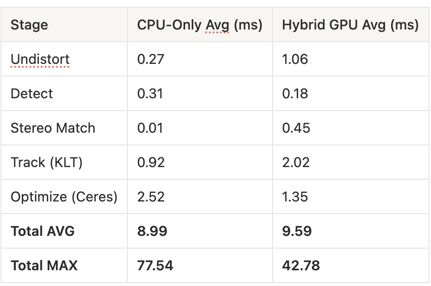
The headline result is not average throughput — it’s latency consistency. The CPU version is slightly faster on average but suffers from massive latency spikes up to 77 ms, violating the 50 ms frame budget at 20 Hz. The GPU version caps worst-case latency at 42 ms, ensuring smooth real-time operation.
A counterintuitive result: the optimization stage drops from 2.52 ms to 1.35 ms on the GPU pipeline, even though Ceres runs identically on both. The Metal FAST + Harris pipeline produces higher-quality corner localizations than OpenCV’s default ORB detector, giving the backend solver better-conditioned data that converges faster.
The GPU undistortion currently shows higher latency than CPU due to getBytes synchronization overhead in the texture readback path. In the production flow, the undistorted texture stays on the GPU (never read back to CPU), so this cost disappears. The profiling numbers reflect the validation path where both GPU and CPU outputs are compared.
9. Conclusion
vio-metal demonstrates that Apple Silicon’s Unified Memory Architecture opens a genuinely different systems design space for real-time perception pipelines. The zero-copy MTLBuffer model eliminates the transfer tax that makes GPU offloading uneconomical on discrete GPU platforms for small, fast kernels. When a kernel runs in 0.1 ms on the GPU and the “upload” is just a pointer cast, offloading becomes viable even when the average throughput gain is negligible — or, as in this case, slightly negative (9.59 ms GPU vs 8.99 ms CPU average).
The real payoff is not in raw speed. It shows up in two places the averages don’t capture. First, latency stability: the GPU pipeline’s worst-case latency of 42 ms versus the CPU’s 77 ms means the difference between hitting and missing the 50 ms frame budget at 20 Hz. For a real-time system, a pipeline that is 0.6 ms slower on average but never spikes past the deadline is strictly better than one that is faster on average but occasionally drops frames. Second, downstream quality: the Metal FAST + Harris front-end produces better-localized corners than OpenCV’s default ORB detector, cutting Ceres optimization time nearly in half (1.35 ms vs 2.52 ms) because the solver converges faster on higher-quality input data. The GPU doesn’t just move computation — it changes the quality of the data flowing into the backend.
The code is open source and available at github.com/MisterEkole/vio-metal.
References
Forster, C., Carlone, L., Dellaert, F., & Scaramanga, D. (2017). “On-Manifold Preintegration for Real-Time Visual-Inertial Odometry.” IEEE Transactions on Robotics, 33(1), 1–21.
Leutenegger, S., Lynen, S., Bosse, M., Siegwart, R., & Furgale, P. (2015). “Keyframe-Based Visual-Inertial Odometry Using Nonlinear Optimization.” IJRR, 34(3), 314–334.
Qin, T., Li, P., & Shen, S. (2018). “VINS-Mono: A Robust and Versatile Monocular Visual-Inertial State Estimator.” IEEE Transactions on Robotics, 34(4), 1004–1020.
Usenko, V., Demmel, N., Schubert, D., Stückler, J., & Cremers, D. (2020). “Visual-Inertial Mapping with Non-Linear Factor Recovery.” IEEE RA-L.
Burri, M., et al. (2016). “The EuRoC Micro Aerial Vehicle Datasets.” IJRR, 35(10), 1157–1163.
Lowe, D. (2004). “Distinctive Image Features from Scale-Invariant Keypoints.” IJCV, 60(2), 91–110.
Rosten, E. & Drummond, T. (2006). “Machine Learning for High-Speed Corner Detection.” ECCV.
Rublee, E., et al. (2011). “ORB: An Efficient Alternative to SIFT or SURF.” ICCV.
Lucas, B. & Kanade, T. (1981). “An Iterative Image Registration Technique with an Application to Stereo Vision.” IJCAI.
Harris, C. & Stephens, M. (1988). “A Combined Corner and Edge Detector.” Alvey Vision Conference.